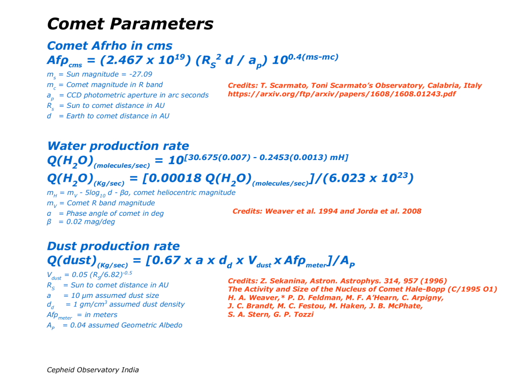
We collected the empirical formulas for comet parameters a like Afρ, Water production rate Q(H2O), (molecules/sec), Dust production rate Q(dust)(Kg/sec) from standard papers and sources with due credits.

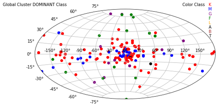
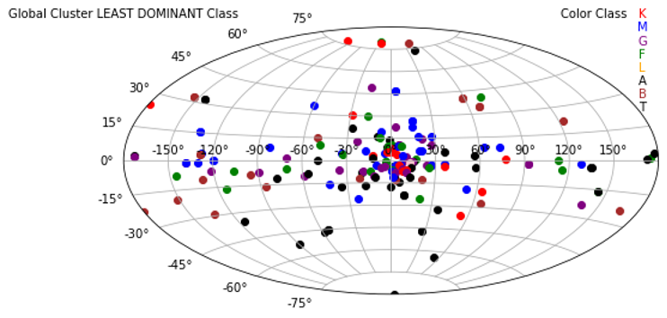
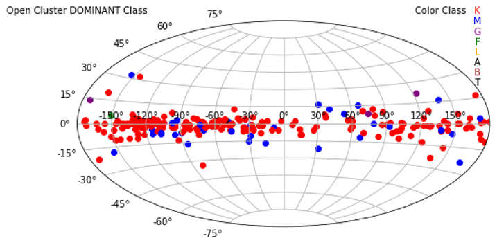
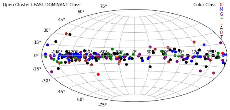
Our friend, Willie Buning, Netherlands, provided the Gaia DR3 data within 30 Kparsec for bright star clusters (Globular as well as open clusters). The table generated by the python code developed by Joseph Karpinski. Willie modified the code a bit for plotting dominated bright star clusters in SQL or Excel. The spectral classification of stars inside clusters and their numbers presented in map. The image of Gaia DR3 map is shown below.

Best spectrophotometric standards:
                                      epoch  mu a cosd  mu d  Class   V Mag

LTT377         00 41 02.9  -33 44 06  1985                    f       11.2
Feige 24       02 32 30.9  +03 30 51  1950   +0.083   +0.010  DAwke   12.42
EG21           03 10 22.1  -68 39 28  1985                    DA      11.4 
G191B2B=EG247  05 01 31.5  +52 45 52  1950   +0.10    -0.0873 DAwk    11.78
GD71           05 49 34.79 +15 52 37  1950   +        -0.1898 DA1     13.03
LTT2415        05 56 24.2  -27 51 26  1985                            12.2
EG54           07 40 19.52 -17 24 41  2000  +1.136"/y -0.52"  DF      12.98 
LTT3218        08 41 33.6  -32 56 55  1985                    DA      11.8
EG63           08 47 29.6  -18 59 50  2000  -0.12"/y -0.05"/y DB      15.55
LTT3864        10 31 33.1  -35 33 03  1985                    f       12.1
Feige 34=EG71  10 36 41.1  +43 21 50  1950                    sdO     11.24
GD153          12 54 35.21 +22 18 09  1950            -0.1898 DA1     13.35
HZ 43 =EG98    13 14 00.7  +29 21 49  1950   -0.149   -0.0813 DAwk    12.91
HZ 44          13 21 19.1  +36 23 38  1950   -0.062   +0.031  sdO     11.67
EG274          16 23 33.7  -39 13 48  2000                    DA      11.0
LTT7379        18 36 26.2  -44 18 37  1985                    G0      10.2
HD 192281      20 10 46.8  +40 07 01  1950                    O5f      7.54
BD+284211=J256 21 48 57.1  +28 37 48  1950                    sdOp    10.56
LTT9239        22 52 40.88 -20 35 26  2000                    f       12.0
Feige110=EG158 23 17 23.5  -05 26 22  1950   +0.003   -0.003  sdO     11.88

OK standards:

Feige 25       02 36 00.0  +05 15 16  1950                    B6V     12.01
Hiltner 600    06 42 37.2  +02 11 25  1950                    B1V     10.42
Feige 56       12 04 13.8  +11 56 55  1950                    B5p     11.11
Feige 92       14 09 41.3  +50 21 07  1950                    Bp      11.62
BD+33 2642     15 50 02.9  +33 05 49  1950                    B2 IVp  10.88
BD+40 4032     20 06 40.0  +41 06 15  1950                    B2 III  10.45

The first set contains O stars without much Balmer absorption plus
faint southern standards from the list of Stone & Baldwin 1983, MN 204, 347.
The second set is mostly B stars that have a bit of Balmer absorption
and are usually OK.

from Link: https://www.cfa.harvard.edu/~dfabricant/huchra/standards.specp

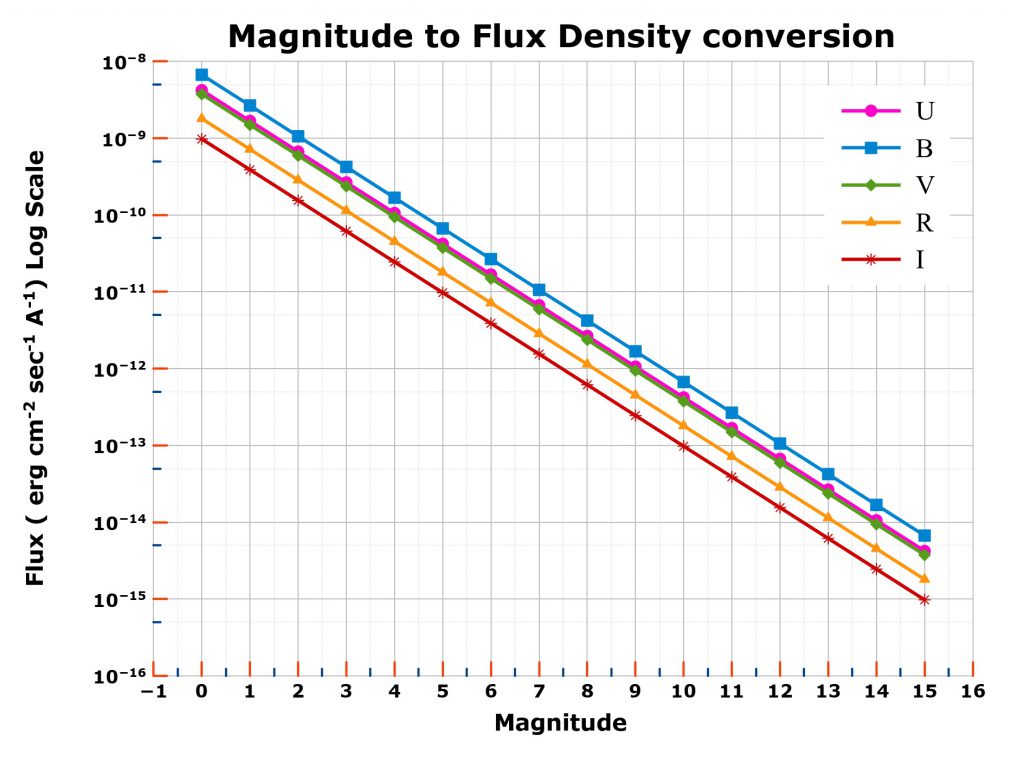
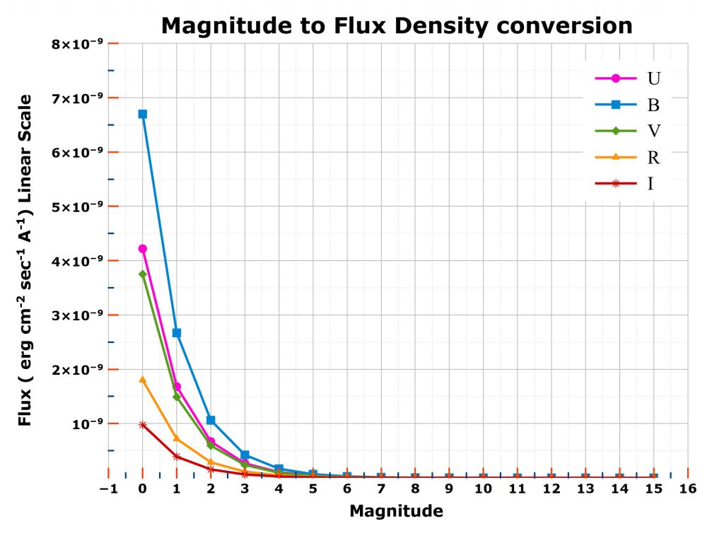
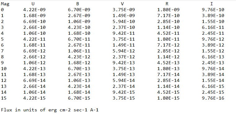
The following graphs shows the conversion of flux densities w.r.t. magnitudes. The magnitude range is selected based on UCAC4 catalog from 0 to +16. The Y axis represents the energy flux in the units of (erg cm^-2 sec^-1 A^-1) w.r.t respective U B V R I magnitudes. The graphs plotted both in Log and Linear scales.

Log Scale:

Linear Scale:

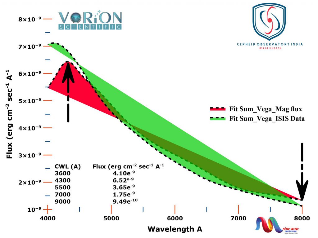
Here is Flux comparison of ISIS data and flux generated by NASA-IPAC tool (https://irsa.ipac.caltech.edu/…/data…/tools/pet/magtojy/) for Vega.Procedure is:1. Flux intensity drag of ISIS data using FIT files>>>then best fitting>>>then plotting w.r.t wavelength.2. Pickup flux intensity using star mag (NASA-IPAC tool) for UBVRI wavelengths>>>then interpolation of all wavelengths points similar to point no. 1>>>then best fitting>>>then plotting w.r.t wavelength. The flux intensity for UBVRI filters at central wavelength are mentioned in graph below.The star magnitude are taken from SIMBAD (but a better catalog may be used if available). In graph, we can compare that energy fluxes are almost similar from range between pointed arrows. The minor difference may be due of some off magnitude of star vega in SIMBAD database or fitting done.We see that fluxes deviate from 4200 A towards UV region. We assume that this is because of fall of CCD sensitivity (silicon band gap, works well from 400nm to 900nm and maintain same sign of slope (dF/dA). We think, this is the reason that, professional astronomers use V/R/I band filter response for absolute flux calibration. We did not find any document where U/B filters response were used for flux calibration. The change of slope of flux vs. wavelength may be a reason (not sure yet).But If We plot from 400nm to 700nm, We find both methods satisfactory. Science is fun!..

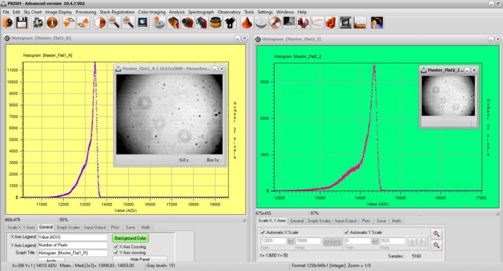
Flat Issues: Tried to analyze the flat frames using PRiSMv10. The CCD Atik383L+ have typical value of full electron well equal to 26,000. Set the diffuser to telescope (3 layered white cloth) and exposed for 1×1 bin and 2×2 bin for different time intervals to get ADU counts near to half of full well capacity. PRiSMv10 analyzed the ADU by plotting each pixel counts under menu: Analysis/Histogram/Global.